

Basic Workflow#
This tutorial walks through a standard single-cell analysis from start to finish: loading data, quality control, feature selection, normalization, dimensionality reduction, clustering, embedding, and marker gene identification.
Dataset#
We use a ~10 million cell cytokine stimulation dataset from Parse Biosciences. Peripheral blood mononuclear cells (PBMCs) from twelve healthy donors were treated with either one of 90 different cytokines or a phosphate-buffered saline (PBS) control for 24 hours, yielding (90 + 1) × 12 = 1,092 experimental conditions.
Download the full single-cell object (~10M cells, 212 GB); the results shown below are for this dataset:
from subprocess import run
run('wget -nc https://parse-wget.s3.us-west-2.amazonaws.com/10m/'
    'Parse_10M_PBMC_cytokines.h5ad',
    shell=True)
Or a subsampled version (~100K cells, 1.5 GB) to follow along on a laptop or other memory-limited machine:
from subprocess import run
run('wget -nc https://huggingface.co/datasets/dashingcell/'
    'Parse_100K_PBMC_cytokines/resolve/main/'
    'Parse_100K_PBMC_cytokines.h5ad',
    shell=True)
Loading data#
SingleCell is brisc’s main class. It represents a single-cell dataset — the count matrix plus metadata for each cell and gene — and provides the methods for working with it.
from brisc import SingleCell
import polars as pl
SingleCell reads and writes the major single-cell formats (.h5ad, .rds, .h5Seurat, .h5, .mtx, .mtx.gz). See Interoperability.
sc = SingleCell(
    'Parse_10M_PBMC_cytokines.h5ad',
    obs_columns=['sample', 'donor', 'cell_type', 'treatment', 'cytokine'])
By default, loading uses all cores available on your machine, as detected by os.cpu_count(). You can change this via the num_threads parameter. num_threads also controls parallelism for every subsequent operation on the dataset. This can be overridden per step (e.g. sc.pca(num_threads=8)) or changed for the dataset as a whole (e.g. sc.num_threads = 8 or sc = sc.set_num_threads(8)).
obs_columns loads only the named metadata columns; omit it to load all of them. For efficiency, we load just the columns used later in the workflow.
For simplicity, speed, and memory efficiency, only a single count matrix is loaded. Because brisc requires the raw counts, we load X from adata.layers['UMIs'] or adata.raw.X if present, and adata.X otherwise. You can override this with the X_key argument to SingleCell.
A quick look at what was loaded:
sc.peek_obs()
 column     value
 _index     89_103_005__s1
 sample     Donor10_4-1BBL
 donor      Donor10
 cell_type  CD8 Naive
 treatment  cytokine
 cytokine   4-1BBL
shape: (6, 2)
sc.peek_var()
 column   value
 _index   TSPAN6
 n_cells  15700
shape: (2, 2)
Inspecting a file before loading
ls() reports an .h5ad file’s dimensions and structure without reading the data. This lets you decide which columns of obs/var to load, and whether to load the count matrix from a custom location (see the X_key argument to SingleCell).
SingleCell.ls('Parse_10M_PBMC_cytokines.h5ad')
X: 9,697,974 × 40,352 sparse array with 18,830,591,942 non-zero elements, data type 'float32', and first non-zero element = 1
obs: _index, bc1_well, bc1_wind, bc2_well, bc2_wind, bc3_well, bc3_wind, cell_type, cytokine, donor, gene_count, log1p_n_genes_by_counts,
     log1p_total_counts, log1p_total_counts_MT, mread_count, pct_counts_MT, sample, species, total_counts_MT, treatment, tscp_count
var: _index, n_cells
Quality control#
This dataset has already been quality-controlled, but we will still run qc() as a demonstration. By default, it keeps cells with:
≤5% mitochondrial reads
≥100 genes detected
non-zero MALAT1 expression — this nuclear lncRNA is ubiquitously expressed, so its absence indicates empty droplets or cytoplasmic fragments.
Like the other steps in this workflow, qc returns a new dataset rather than changing it in place, so we assign the result back to sc.
sc = sc.qc(allow_float=True, verbose=True)
Starting with 9,697,974 cells.
Filtering to cells with ≤5.0% mitochondrial counts...
9,443,200 cells remain after filtering to cells with ≤5.0% mitochondrial counts.
Filtering to cells with ≥100 genes detected (with non-zero count)...
9,443,200 cells remain after filtering to cells with ≥100 genes detected.
Filtering to cells with non-zero MALAT1 expression...
9,443,163 cells remain after filtering to cells with non-zero MALAT1 expression.
Adding a Boolean column, obs['passed_QC'], indicating which cells passed QC...
qc() expects raw integer counts and will raise an error when they are floating-point, to protect you from accidentally running QC on normalized data. However, this dataset’s raw counts happen to be stored as float32 (which is quite common), so we pass allow_float=True to bypass the error. This is only safe when the values are genuinely raw counts.
By default, qc() does not actually filter out any cells; it merely adds a Boolean column (called passed_QC by default) to obs, where cells that pass QC are flagged as True. brisc’s downstream methods then look at this column (or more specifically, the column specified by their QC_column arguments, which also default to passed_QC) to skip QC-failing cells. This trick roughly halves brisc’s peak memory usage, but requires special care when interacting with external pipelines that do not recognize this QC column. To remove QC-failing cells entirely, like Scanpy and Seurat do, specify subset=True during QC.
print(sc.obs)
shape: (9_697_974, 7)
┌──────────────────┬────────────────┬─────────┬───────────────────────┬───────────┬──────────┬───────────┐
│ _index           ┆ sample         ┆ donor   ┆ cell_type             ┆ treatment ┆ cytokine ┆ passed_QC │
│ ---              ┆ ---            ┆ ---     ┆ ---                   ┆ ---       ┆ ---      ┆ ---       │
│ str              ┆ enum           ┆ enum    ┆ enum                  ┆ enum      ┆ enum     ┆ bool      │
╞══════════════════╪════════════════╪═════════╪═══════════════════════╪═══════════╪══════════╪═══════════╡
│ 89_103_005__s1   ┆ Donor10_4-1BBL ┆ Donor10 ┆ CD8 Naive             ┆ cytokine  ┆ 4-1BBL   ┆ true      │
│ 89_103_083__s1   ┆ Donor10_4-1BBL ┆ Donor10 ┆ B Naive               ┆ cytokine  ┆ 4-1BBL   ┆ true      │
│ 89_103_085__s1   ┆ Donor10_4-1BBL ┆ Donor10 ┆ B Intermediate/Memory ┆ cytokine  ┆ 4-1BBL   ┆ false     │
│ 89_104_009__s1   ┆ Donor10_4-1BBL ┆ Donor10 ┆ CD14 Mono             ┆ cytokine  ┆ 4-1BBL   ┆ true      │
│ 89_104_025__s1   ┆ Donor10_4-1BBL ┆ Donor10 ┆ CD14 Mono             ┆ cytokine  ┆ 4-1BBL   ┆ true      │
│ …                ┆ …              ┆ …       ┆ …                     ┆ …         ┆ …        ┆ …         │
│ 61_186_093__s144 ┆ Donor9_VEGF    ┆ Donor9  ┆ CD4 Memory            ┆ cytokine  ┆ VEGF     ┆ true      │
│ 61_186_108__s144 ┆ Donor9_VEGF    ┆ Donor9  ┆ CD14 Mono             ┆ cytokine  ┆ VEGF     ┆ true      │
│ 61_186_135__s144 ┆ Donor9_VEGF    ┆ Donor9  ┆ CD8 Naive             ┆ cytokine  ┆ VEGF     ┆ true      │
│ 61_186_157__s144 ┆ Donor9_VEGF    ┆ Donor9  ┆ CD8 Naive             ┆ cytokine  ┆ VEGF     ┆ true      │
│ 61_186_168__s144 ┆ Donor9_VEGF    ┆ Donor9  ┆ B Intermediate/Memory ┆ cytokine  ┆ VEGF     ┆ true      │
└──────────────────┴────────────────┴─────────┴───────────────────────┴───────────┴──────────┴───────────┘
Exploring QC metrics
To facilitate more in-depth exploration of data quality before filtering, qc_metrics() adds num_counts, num_genes, and mito_fraction columns to obs. This is optional, since qc() calculates its own filters internally.
sc = sc.qc_metrics(allow_float=True)
print(sc.obs.select('num_counts', 'num_genes', 'mito_fraction').describe())
┌────────────┬─────────────┬─────────────┬───────────────┐
│ statistic  ┆ num_counts  ┆ num_genes   ┆ mito_fraction │
│ ---        ┆ ---         ┆ ---         ┆ ---           │
│ str        ┆ f64         ┆ f64         ┆ f64           │
╞════════════╪═════════════╪═════════════╪═══════════════╡
│ count      ┆ 9.697974e6  ┆ 9.697974e6  ┆ 9.697974e6    │
│ null_count ┆ 0.0         ┆ 0.0         ┆ 0.0           │
│ mean       ┆ 4372.856645 ┆ 1941.703694 ┆ 0.020779      │
│ std        ┆ 3870.176441 ┆ 934.460866  ┆ 0.01191       │
│ min        ┆ 436.0       ┆ 399.0       ┆ 0.0           │
│ 25%        ┆ 2014.0      ┆ 1274.0      ┆ 0.012927      │
│ 50%        ┆ 3320.0      ┆ 1795.0      ┆ 0.018277      │
│ 75%        ┆ 5379.0      ┆ 2417.0      ┆ 0.025636      │
│ max        ┆ 70055.0     ┆ 7000.0      ┆ 0.149981      │
└────────────┴─────────────┴─────────────┴───────────────┘
Customizing QC
Each QC threshold is configurable:
sc = sc.qc(max_mito_fraction=0.10, min_genes=200, nonzero_MALAT1=False, allow_float=True)
custom_filter adds an extra per-cell filter on top of these: pass a Boolean polars expression or column name to force cells where the custom filter is False to fail QC.
Removing doublets
brisc uses the fast cxds algorithm for doublet detection. Doublet removal is off by default, and we skip it here because this dataset’s doublets were already removed, and it would be invalid to perform doublet detection twice. To add doublet detection to the QC filtering, specify remove_doublets=True. Specify batch_column to perform doublet detection independently within each sequencing batch:
sc = sc.qc(remove_doublets=True, batch_column='sample', allow_float=True)
Doublet detection can also be run as a standalone step, via find_doublets(). It adds doublet and doublet_score columns to obs for you to inspect or threshold yourself. This should only be run after all other QC filters have been applied.
sc = sc.find_doublets(batch_column='sample')
Skipping QC
Duplicate cell or gene names
qc() raises an error if any name appears more than once in obs_names or var_names. Deduplicate first with make_obs_names_unique() or make_var_names_unique(), which append -1, -2, … to repeated names:
sc = sc.make_var_names_unique()
Feature selection#
hvg() selects highly variable genes using the same approach as Seurat’s FindVariableFeatures(). It operates on raw counts and must be run before normalize(). By default, it selects the top 2,000 genes.
When your data has multiple batches, pass batch_column to identify genes that are consistently variable across batches:
sc = sc.hvg(batch_column='donor')
This adds highly_variable and highly_variable_rank columns to var. pca() then uses only these genes, and the steps after it build on the resulting PCs.
print(sc.var.filter('highly_variable').sort('highly_variable_rank'))
shape: (2_000, 4)
┌─────────────────┬─────────┬─────────────────┬──────────────────────┐
│ _index          ┆ n_cells ┆ highly_variable ┆ highly_variable_rank │
│ ---             ┆ ---     ┆ ---             ┆ ---                  │
│ str             ┆ i64     ┆ bool            ┆ u32                  │
╞═════════════════╪═════════╪═════════════════╪══════════════════════╡
│ IGHA1           ┆ 193374  ┆ true            ┆ 1                    │
│ IGKC            ┆ 814041  ┆ true            ┆ 2                    │
│ CEMIP           ┆ 666595  ┆ true            ┆ 3                    │
│ ZNF385D         ┆ 141736  ┆ true            ┆ 4                    │
│ FN1             ┆ 230969  ┆ true            ┆ 5                    │
│ …               ┆ …       ┆ …               ┆ …                    │
│ CDH15           ┆ 2021    ┆ true            ┆ 1996                 │
│ CD84            ┆ 3640179 ┆ true            ┆ 1997                 │
│ KLRC2           ┆ 383626  ┆ true            ┆ 1998                 │
│ ENSG00000283648 ┆ 189431  ┆ true            ┆ 1999                 │
│ ENSG00000254092 ┆ 34573   ┆ true            ┆ 2000                 │
└─────────────────┴─────────┴─────────────────┴──────────────────────┘
Note
polars supports 3 ways of referencing columns: .filter('highly_variable'), .filter(pl.col.highly_variable), and .filter(pl.col('highly_variable')) are all equivalent. The last two are very flexible (e.g. .filter(pl.col.a == pl.col.b), .filter(pl.col('c') >= 0)), and the last one is most flexible since it supports column names with spaces or other characters that would be invalid in Python variable names.
Normalization#
normalize() corrects for differences in sequencing depth, then log-transforms the counts. The default method, log1pPF (Ahlmann-Eltze and Huber 2023), scales each cell by its library size relative to the mean library size (“proportional fitting”) before applying a log1p (y = log(x + 1)) transformation. With method='PFlog1pPF', a second round of proportional fitting is applied after log1p (Booeshaghi et al. 2022). With method='logCP10k', it matches Seurat’s NormalizeData().
sc = sc.normalize()
Note
On large datasets, pass inplace=True to normalize the counts in place instead of allocating a new count matrix, reducing the peak memory of this step. In-place normalization requires a float32 count matrix (as this dataset has) and raises an error for any other data type.
sc = sc.normalize(inplace=True)
PCA#
pca() computes principal components from the normalized, highly variable genes, storing them in obsm['pca']. The default num_PCs is 50.
sc = sc.pca()
Note
When running single-threaded (num_threads=1), brisc’s PCA defaults to a different order of operations than the multi-threaded path. It’s roughly twice as fast and uses less memory, but the floating-point output differs slightly from the multi-threaded run. Pass match_parallel=True (only valid with num_threads=1) to get identical results to a multi-threaded run:
sc = sc.pca(num_threads=1, match_parallel=True)
Integrating batches
If your data spans several batches (different samples, donors, or runs), integrate them by adding harmonize() after PCA — it removes the batch differences from the PCs into obsm['harmony']. When doing this, specify PC_key='harmony' to all subsequent steps that require PCs, so that they use the harmonized PCs instead of the raw ones:
To integrate separate datasets — for example, mapping an annotated reference onto a query — see Integration and Label Transfer.
Nearest neighbors#
brisc builds a neighbor graph in two steps:
neighbors() finds each cell’s num_neighbors (default 20) nearest neighbors using a fast approximate search, storing their indices in obsm['neighbors'] and the squared Euclidean distances in obsm['distances'].
shared_neighbors() then builds the shared nearest neighbor (SNN) graph, connecting two cells in proportion to how many neighbors they share, and stores it in obsp['shared_neighbors'].
sc = sc.neighbors().shared_neighbors()
Note
If you subset your data after computing neighbors (e.g. via filter_obs()), the neighbor graph becomes invalid and must be recomputed. brisc will detect this and raise an error.
Clustering#
cluster() runs Leiden clustering on the SNN graph. The resolution parameter controls granularity — higher values produce more clusters. You can pass multiple resolutions to evaluate them in parallel:
sc = sc.cluster(resolution=[0.25, 0.5, 1.0, 1.5, 2.0])
Each resolution adds a column to obs: cluster_0 through cluster_4 (the prefix 'cluster' can be changed by specifying cluster_column).
Embedding#
To visualize the data, brisc embeds the cells in two dimensions. Most single-cell workflows use UMAP:
sc = sc.umap()
Embeddings are stored as 2-column NumPy arrays in obsm (here, obsm['umap']). plot_umap() colors the embedding by an obs column and saves it to a file, or shows it interactively if you omit the filename:
sc.plot_umap('cell_type', 'umap.png')
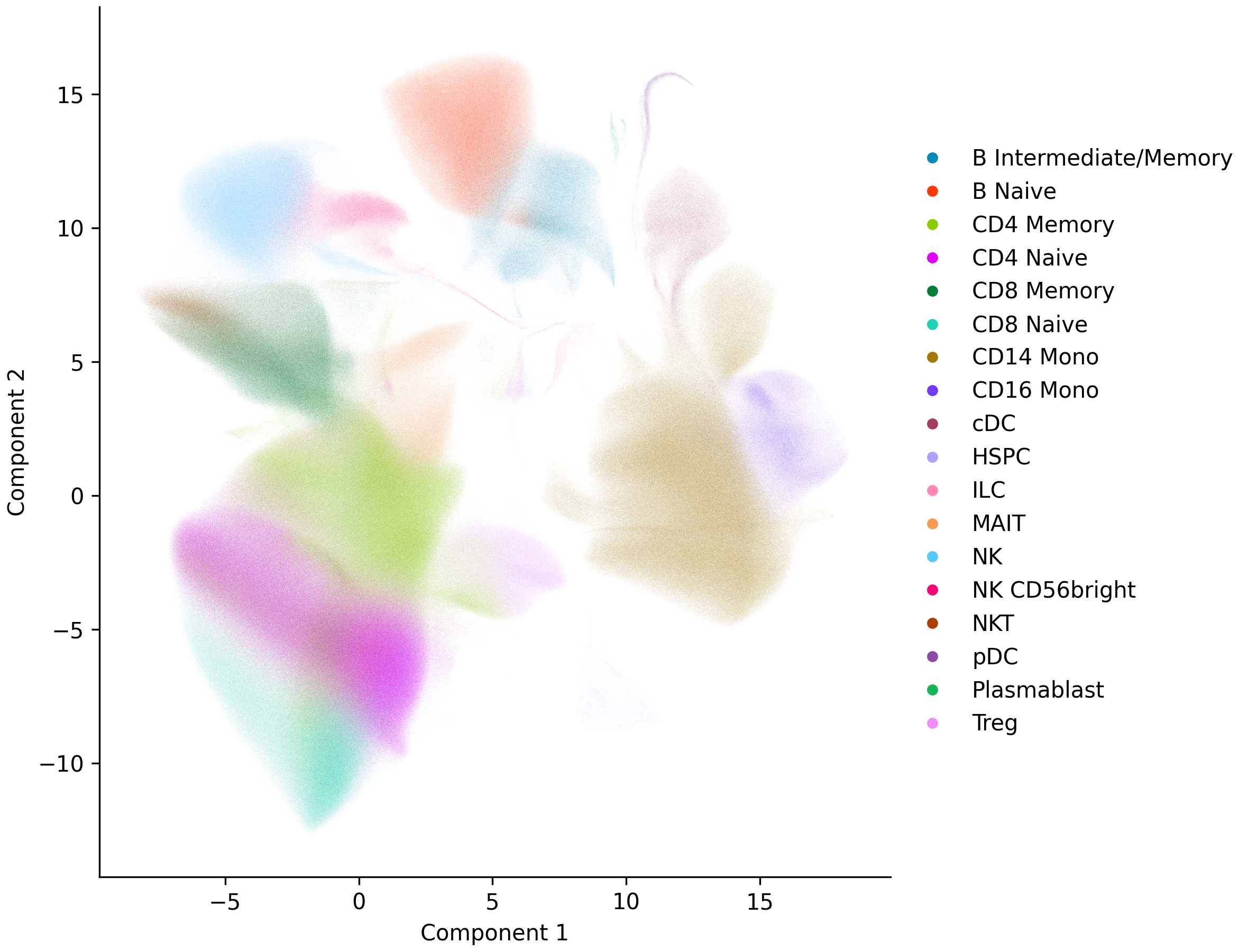
UMAP is the slowest of brisc’s embeddings, and there are two ways to go faster. To speed up UMAP itself, pass hogwild=True, which parallelizes its otherwise single-threaded optimization with Hogwild! gradient descent — much faster, but no longer reproducible, with runs varying slightly even at a fixed seed.
Or switch to a faster method: pacmap() (PaCMAP), a relative of UMAP that also captures global structure better, or localmap() (LocalMAP), a newer relative of PaCMAP that further sharpens local cluster separation. Each has its own plotter — plot_pacmap() and plot_localmap().
Marker genes#
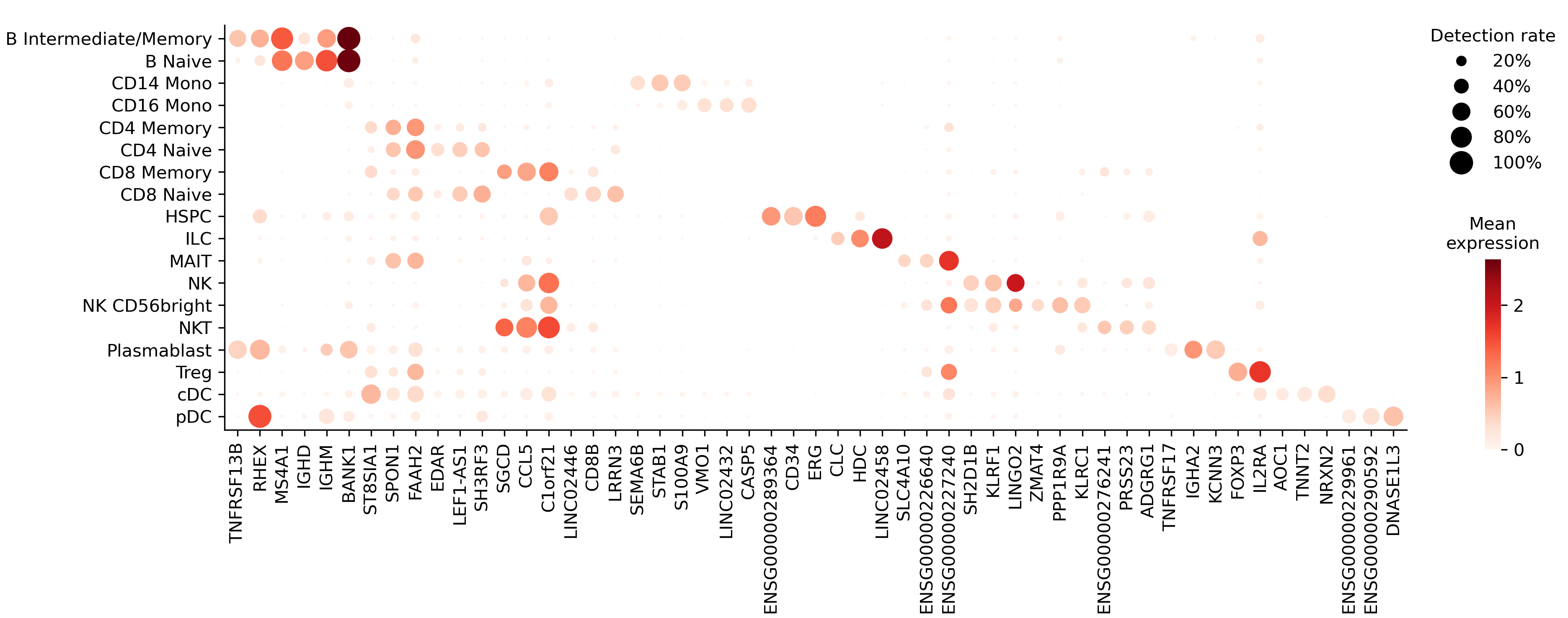
find_markers() finds each cell type’s marker genes — those that distinguish it from all other cell types. Adapted from Fischer and Gillis 2021, it scores genes by their detection rate within the type and the fold change in detection rate against the others. It uses only whether each gene is detected, not how strongly, so raw and normalized counts give the same result.
Here, we use the dataset’s precomputed cell-type labels (the cell_type column) to define markers. In a real workflow, you would run find_markers() on the Leiden clusters from cluster(), and use the markers to manually annotate each cell type. Or, you might use label transfer from a reference atlas to guide the annotation of the Leiden clusters — see Integration and Label Transfer.
markers = sc.find_markers('cell_type')
markers comes sorted by descending fold change, so grouping by cell_type and taking head(3) — with maintain_order=True to preserve that order — gives the three strongest markers per type:
top = markers.group_by('cell_type', maintain_order=True).head(3)
print(top)
shape: (53, 4)
┌───────────────────────┬─────────────────┬────────────────┬─────────────┐
│ cell_type             ┆ gene            ┆ detection_rate ┆ fold_change │
│ ---                   ┆ ---             ┆ ---            ┆ ---         │
│ enum                  ┆ str             ┆ f32            ┆ f32         │
╞═══════════════════════╪═════════════════╪════════════════╪═════════════╡
│ B Intermediate/Memory ┆ TNFRSF13B       ┆ 0.520794       ┆ 82.767754   │
│ B Intermediate/Memory ┆ RHEX            ┆ 0.586154       ┆ 25.334995   │
│ B Intermediate/Memory ┆ MS4A1           ┆ 0.8869         ┆ 15.144114   │
│ B Naive               ┆ IGHD            ┆ 0.646712       ┆ 59.548691   │
│ B Naive               ┆ IGHM            ┆ 0.849442       ┆ 30.27688    │
│ B Naive               ┆ BANK1           ┆ 0.973336       ┆ 11.047324   │
│ CD4 Memory            ┆ ST8SIA1         ┆ 0.267901       ┆ 3.107528    │
│ CD4 Memory            ┆ SPON1           ┆ 0.435606       ┆ 2.597597    │
│ CD4 Memory            ┆ FAAH2           ┆ 0.564531       ┆ 2.124807    │
│ CD4 Naive             ┆ EDAR            ┆ 0.326444       ┆ 8.546687    │
│ CD4 Naive             ┆ LEF1-AS1        ┆ 0.411832       ┆ 5.044062    │
│ CD4 Naive             ┆ SH3RF3          ┆ 0.41861        ┆ 4.286712    │
│ CD8 Memory            ┆ SGCD            ┆ 0.395334       ┆ 11.698642   │
│ CD8 Memory            ┆ CCL5            ┆ 0.616458       ┆ 7.031501    │
│ CD8 Memory            ┆ C1orf21         ┆ 0.666685       ┆ 5.679882    │
│ CD8 Naive             ┆ LINC02446       ┆ 0.33037        ┆ 23.228165   │
│ CD8 Naive             ┆ CD8B            ┆ 0.432123       ┆ 11.777583   │
│ CD8 Naive             ┆ LRRN3           ┆ 0.493111       ┆ 9.237646    │
│ CD14 Mono             ┆ SEMA6B          ┆ 0.383729       ┆ 89.544785   │
│ CD14 Mono             ┆ STAB1           ┆ 0.520267       ┆ 70.046577   │
│ CD14 Mono             ┆ S100A9          ┆ 0.522546       ┆ 43.416138   │
│ CD16 Mono             ┆ VMO1            ┆ 0.35694        ┆ 33.207912   │
│ CD16 Mono             ┆ LINC02432       ┆ 0.357715       ┆ 27.628471   │
│ CD16 Mono             ┆ CASP5           ┆ 0.422475       ┆ 18.697172   │
│ HSPC                  ┆ ENSG00000289364 ┆ 0.62795        ┆ 3727.717285 │
│ HSPC                  ┆ CD34            ┆ 0.632067       ┆ 489.117584  │
│ HSPC                  ┆ ERG             ┆ 0.810472       ┆ 367.071747  │
│ ILC                   ┆ CLC             ┆ 0.328625       ┆ 1614.022095 │
│ ILC                   ┆ HDC             ┆ 0.571653       ┆ 860.066284  │
│ ILC                   ┆ LINC02458       ┆ 0.767234       ┆ 143.109436  │
│ MAIT                  ┆ SLC4A10         ┆ 0.284689       ┆ 41.925579   │
│ MAIT                  ┆ ENSG00000226640 ┆ 0.343954       ┆ 14.488205   │
│ MAIT                  ┆ ENSG00000227240 ┆ 0.712267       ┆ 7.911214    │
│ NK                    ┆ SH2D1B          ┆ 0.445389       ┆ 62.467659   │
│ NK                    ┆ KLRF1           ┆ 0.514243       ┆ 23.452459   │
│ NK                    ┆ LINGO2          ┆ 0.584149       ┆ 21.811985   │
│ NK CD56bright         ┆ ZMAT4           ┆ 0.275323       ┆ 66.026596   │
│ NK CD56bright         ┆ PPP1R9A         ┆ 0.463418       ┆ 34.774734   │
│ NK CD56bright         ┆ KLRC1           ┆ 0.485791       ┆ 20.565966   │
│ NKT                   ┆ ENSG00000276241 ┆ 0.3314         ┆ 20.063036   │
│ NKT                   ┆ PRSS23          ┆ 0.362412       ┆ 17.436337   │
│ NKT                   ┆ ADGRG1          ┆ 0.363574       ┆ 13.671699   │
│ Plasmablast           ┆ TNFRSF17        ┆ 0.293468       ┆ 724.194092  │
│ Plasmablast           ┆ IGHA2           ┆ 0.585975       ┆ 232.649841  │
│ Plasmablast           ┆ KCNN3           ┆ 0.636167       ┆ 150.661896  │
│ Treg                  ┆ FOXP3           ┆ 0.631336       ┆ 91.637367   │
│ Treg                  ┆ IL2RA           ┆ 0.839082       ┆ 14.339853   │
│ cDC                   ┆ AOC1            ┆ 0.288216       ┆ 621.899048  │
│ cDC                   ┆ TNNT2           ┆ 0.396086       ┆ 430.963531  │
│ cDC                   ┆ NRXN2           ┆ 0.537554       ┆ 356.248749  │
│ pDC                   ┆ ENSG00000229961 ┆ 0.354319       ┆ 9908.68457  │
│ pDC                   ┆ ENSG00000290592 ┆ 0.517426       ┆ 4866.669434 │
│ pDC                   ┆ DNASE1L3        ┆ 0.704335       ┆ 1133.133545 │
└───────────────────────┴─────────────────┴────────────────┴─────────────┘
Each row is a marker gene. detection_rate is the fraction of that cell type’s cells in which the gene is detected; fold_change is how much more often it’s detected in that type than elsewhere. A gene must first clear both thresholds — detection_rate ≥ 0.25 (min_detection_rate) and fold_change ≥ 2 (min_fold_change). Because the two trade off against each other, brisc then keeps only the genes on their Pareto front — those no other gene beats on both at once. Pass pareto=False to keep every gene that clears the thresholds instead.
The table holds only marker genes; pass all_genes=True to include every gene, with a marker column flagging the selected ones.
plot_markers() draws a dot plot of chosen genes across cell types, sizing each dot by detection rate and coloring it by expression (or by fold change with color='fold_change'):
sc.plot_markers(top['gene'], 'cell_type', 'markers.png')
Saving#
save() writes to multiple supported formats: .h5ad, .rds, .h5Seurat, .h5, .mtx, or .mtx.gz. See Interoperability.
It won’t overwrite an existing file unless you pass overwrite=True.
sc.save('processed.h5ad', overwrite=True)
Because our QC didn’t subset the data (subset defaults to False), the saved file includes every cell, with passed_QC flagging the ones that passed. To save only those cells, run qc() with subset=True, or filter the dataset first:
sc.filter_obs('passed_QC').save('processed.h5ad', overwrite=True)
Pipeline summary#
Because each method returns a new dataset, the full pipeline chains together:
sc = SingleCell('Parse_10M_PBMC_cytokines.h5ad', num_threads=-1)\
    .qc(allow_float=True)\
    .hvg(batch_column='donor')\
    .normalize()\
    .pca()\
    .neighbors()\
    .shared_neighbors()\
    .cluster(resolution=[0.25, 0.5, 1.0, 1.5, 2.0])\
    .umap()

sc.plot_umap('cell_type', 'umap.png')
markers = sc.find_markers('cell_type')
top = markers.group_by('cell_type', maintain_order=True).head(3)
sc.plot_markers(top['gene'], 'cell_type', 'markers.png')
sc.save('Parse_10M_PBMC_cytokines_processed.h5ad', overwrite=True)
Step |
Method |
What it does |
|---|---|---|
Load |
Read data from any supported format |
|
Quality control |
Filter low-quality cells |
|
Feature selection |
Select highly variable genes |
|
Normalization |
Normalize and log-transform with log1pPF |
|
PCA |
Compute principal components |
|
Neighbors |
Find each cell’s nearest neighbors |
|
Shared neighbors |
Build the shared nearest neighbor graph |
|
Clustering |
Cluster with Leiden at one or more resolutions |
|
Embedding |
Embed in 2D for visualization (UMAP, PaCMAP, or LocalMAP) |
|
Plot embedding |
Plot an embedding |
|
Markers |
Find marker genes for each cell type |
|
Plot markers |
Draw a dot plot of marker genes |
|
Save |
Write to |